The math behind the lookAt() transform

In computer graphics, one of the key elements of the graphics pipeline is the View transformation, which is used in the vertex shading stage to convert coordinates from World space to View space. The View transform is usually constructed using a utility function like glm::lookAt() from the GLM library, or D3DXMatrixLookAtLH() in DirectX. But what are these functions actually doing? In this post we will do a deep dive into the math behind the glm::lookAt() function. This will also serve as a way to understand and put into practice some important concepts of linear algebra and geometry.

Before we go into the actual explanation, we need to lay some mathematical groundwork first.

The change of basis matrix

Theorem: consider the $\mathbb{R}^n$ vector space and two bases $SRC$ and $DST$ . The function that takes the coordinates of a vector in $SRC$ and converts them into coordinates of the same vector in $DST$ is a linear transformation and its associated matrix $_{DST}M_{SRC}$ is composed of the coordinates of the vectors of $SRC$ expressed in $DST$ , placed as columns.

For the proof of this theorem see Sources. It’s the best explanation I’ve seen of the subject, rigorous and also elegant.

Key takeaways:

In the above theorem it’s irrelevant which of the two bases represents the source and which represents the destination. We can swap them and the statement still holds. This means that if we want to convert coordinates in $DST$ to coordinates in $SRC$ , the basis change matrix is built by taking the coordinates of the $DST$ vectors expressed in $SRC$ and placing them as columns.
The basis change matrix from $DST$ to $SRC$ $_{SRC}M_{DST}$ can also be obtained as the inverse of the basis change from $SRC$ to $DST$ $_{DST}M_{SRC}$ . That is, $_{SRC}M_{DST} = {_{DST}M_{SRC}}^-1$
An interesting special case is when $SRC$ is the canonical basis and $DST$ is orthonormal. In this case the basis change matrix $_{DST}M_{SRC}$ can be built without doing any calculation at all. In effect, let’s start the other way around and build $_{SRC}M_{DST}$ . In order to do this, we need to obtain the coordinates of the $DST$ vectors expressed in $SRC$ and put them as columns. But since $SRC$ is the canonical base, these coordinates are just the tuples of $DST$ as column vectors. The matrix $_{DST}M_{SRC}$ is the inverse of $_{SRC}M_{DST}$ , but since $DST$ is an orthonormal base, it means the matrix $_{SRC}M_{DST}$ is an orthogonal matrix, and so its inverse is its transpose. In other words, in the special case when $SRC$ is the canonical basis and $DST$ is orthonormal, the basis change matrix $_{DST}M_{SRC}$ can be built by taking the vectors if $DST$ and placing them as rows. Keep this in mind for later.

Geometric interpretation of the change of basis matrix

Although not directly related to the lookAt function, there is an interesting geometric observation that we can make from the above theorem.

Consider the change of basis matrix from $DST$ to $SRC$ , $_{SRC}M_{DST}$ . Take the first vector of $SRC$ , and take its coordinates in $SRC$ . This is the vector $(1, 0, ..., 0)$ . If we multiply this vector by $_{SRC}M_{DST}$ , what we get is a linear combination of the columns of the matrix using the elements of the vector as coefficients. But since the vector is all zeroes except for the first element, this matrix-vector multiplication will yield the first column of the matrix, which is made of the coordinates of the first vector of $DST$ expressed in $SRC$ . Following this argument for the rest of the vectors of $SRC$ , we can see that $_{SRC}M_{DST}$ is also the associated matrix of the transform T that takes $SRC$ into $DST$ . Symbolically:

$_{SRC}M_{DST} = _{SRC}((T))_{SRC}$

Taking inverse on both sides of the equation we get:

${_{SRC}M_{DST}}^{-1} = {_{SRC}((T))_{SRC}}^{-1}$

$_{DST}M_{SRC} = _{SRC}((T^{-1}))_{SRC}$

It is worth noting that the two matrices in the equation are expressed in different bases: the left side is a matrix that takes coordinates in $SRC$ and returns coordinates in $DST$ , whereas the right hand side is a matrix that takes coordinates in $SRC$ and returns coordinates in $SRC$ .

This is the geometric interpretation of the change of basis transform: converting coordinates in $SRC$ to coordinates in $DST$ is equivalent to taking the vector represented by the coordinates in $SRC$ , transforming it with the inverse of the transform that turns $SRC$ into $DST$ , and interpreting the resulting tuple as if they were coordinates in $DST$ .

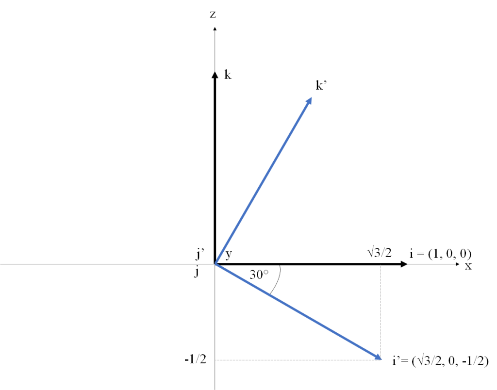
To get an intuitive understanding of this observation, let’s use an example. Consider $\mathbb{R}^3$ , let $SRC$ be the canonical basis and $T$ be a rotation of 30 degrees counterclockwise around the $-Y$ axis. The $DST$ basis is the result of applying $T$ to the vectors of $SRC$ .

Say we want to compute the coordinates of $i$ in $DST$ . One way of doing it is to leave the vector $i$ fixed, rotate the basis $SRC$ so that it becomes $DST$ and then project $i$ onto the direction of the rotated basis vectors. The coordinates of $i$ in $DST$ , which we will denote as $[i]_{DST}$ , are $(\sqrt{3}/2, 0, -1/2)$ . Figure 1 illustrates this approach. We are using a right-handed coordinate system (Y points into the screen). The vectors of the canonical basis $SRC$ are represented as $i$ , $j$ , and $k$ , show in black. The rotated vectors of $DST$ are $i'$ , $j'$ and $k'$ , shown in blue (note the $j$ vector remains fixed due to the axis of the rotation being parallel to it).

Figure 1. Visualizing the coordinates of i in DST. The vector i is fixed and the basis is rotated counterclockwise

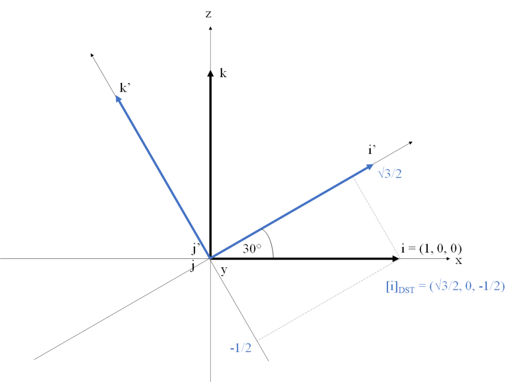
Alternatively, we can leave the basis fixed and rotate the vector $i$ 30 degrees clockwise (i.e. applying the inverse of $T$ ). The coordinates we obtain are the same. Figure 2 illustrates this process.

Figure 2. The SRC basis is fixed and we rotate i clockwise.

Projection of a vector onto another vector

Given a vector space $V$ and a vector $a$ in $V$ , the projection of $a$ onto a nonzero vector $b$ is the vector colinear with $b$ that minimizes the length of $a - b$ .

The projection of $a$ onto $b$ can be computed as $(\frac{a . b}{|| b ||^2}) b$ .

This is related to the concept of coordinates. Given a base $B = \{v_1, v_2, ..., v_n\}$ of $V$ , the coordinates of $a$ with respect to $B$ are the $\lambda_i = \frac{a . v_i}{|| v_i ||^2}$ .

An interesting special case is when all the $v_i$ are of length 1. In that case the coefficients becomes simply $\lambda_i = a . v_i$ .

Affine spaces and affine frames

The affine space is an algebraic structure that provides a natural abstraction to represent physical space. Informally, an affine space is an extension of a vector space where we add a set of points to distinguish them from vectors. The set of points doesn’t have an origin, and points cannot be added together, but a point can be added to a vector (sometimes called displacement vector) to yield another point which represents the translation of the point by the vector. Similarly, two points can be subtracted to give a displacement vector.

Given two affine spaces $X$ and $Z$ , a function $f: X \rightarrow Z$ is an affine map if there exists a linear map $m_f$ such that $f(x) - f(y) = m_f(x - y)$ for all $x, y$ in $X$ . Affine maps are functions that preserve lines and parallelism, while not necessarily preserving lengths and angles. All linear maps can be seen as special cases of affine maps, but not all affine maps are linear maps, because affine maps are not constrained to map the origin to the origin.

The set of points of an affine space doesn’t have an origin. In order to describe the coordinates of a point, we must arbitrarily define a point as origin and describe the coordinates of the displacement vectors relative to that origin. An affine frame is composed of a point $o$ that we call origin and a basis $B = \{v_1, v_2, ..., v_n\}$ of the vector space.

Given a frame $(o, v_1, v_2, ..., v_n)$ for each point $p$ there is a unique set of coefficients $\lambda_i$ such that:

$p - o = \lambda_1v_1 + \lambda_2v_2 + ... + \lambda_nv_n$

The $\lambda_i$ are called the affine coordinates of $p$ in the frame $(o, v_1, v_2, ..., v_n)$ .

Note that although the point set of an affine space doesn’t have the concept of an origin point, we can always arbitrarily choose an affine frame, and this allows us to represent any point by its coordinates in that frame.

For a more formal and detailed description of the concepts of affine space and affine frame, see Sources.

Homogeneous coordinates

For an in-depth description of homogeneous coordinates and how they work, see see Sources.

What follows are the key takeaways of the subject, without going into much formality.

Every affine map can be represented as the composition of a linear map and a translation.

An affine map from $\mathbb{R}^3 \rightarrow \mathbb{R}^3$ cannot be described by a 3×3 matrix, because it’s not a linear map (it has a translation component).

Homogeneous coordinates allow us to represent an affine map in $\mathbb{R}^3 \rightarrow \mathbb{R}^3$ as a 4×4 matrix.

Given an affine map $f: \mathbb{R}^3 \rightarrow \mathbb{R}^3$ which is a composition of linear map $r$ and a translation $t$ by a vector $(t_x, t_y, t_z)$ (that is $f = t ^ {\circ} r$ ), $f$ can be represented by a 4×4 matrix $M$ . To compute the matrix $M$ , let

$R = \begin{pmatrix} R_{11} & R_{12} & R_{13} & 0\\ R_{21} & R_{22} & R_{23} & 0\\ R_{31} & R_{32} & R_{33} & 0\\ 0 & 0 & 0 & 1 \end{pmatrix}$

(The upper-left components of $R$ are taken from the associated matrix of $r$ ).

Let

$T = \begin{pmatrix} 1 & 0 & 0 & t_x \\ 0 & 1 & 0 & t_y\\ 0 & 0 & 1 & t_z\\ 0 & 0 & 0 & 1 \end{pmatrix}$

Then

$M = T * R = \begin{pmatrix} R_{11} & R_{12} & R_{13} & t_x\\ R_{21} & R_{22} & R_{23} & t_y\\ R_{31} & R_{32} & R_{33} & t_z\\ 0 & 0 & 0 & 1 \end{pmatrix}$

(Note $R$ is applied first, then $T$ ).

In order to transform a point $p = (x, y, z)$ by an affine map $f$ , first we convert $p$ to an $\mathbb{R}^4$ column vector in homogeneous coordinates $p_h = (x, y, z, 1)$ (setting its $w$ component to 1), compute the matrix-vector multiplication $p_h' = (x', y', z', w) = M * p_h$ , then we convert $p_h'$ back to $\mathbb{R}^3$ by dividing its first three components by the fourth: $f(p) = (x'/w, y'/w, z'/w)$ .

Define and be aware of your coordinate systems orientation

In order to build the view matrix, you will first need to choose the handedness of the world and view coordinate systems and the orientation of the camera in the view system. In theory, this choice is up to the programmer and doesn’t depend on the graphics API you are using. Graphics APIs don’t care about what coordinate systems you use for the world and view spaces. What they specify is the handedness and range of the Normalized Device Coordinate (NDC) system and the orientation of the camera in it. You are free to choose the model, world and view coordinate systems however you want as long as you build the model, view and projection matrices in such a way that the $P * V * M$ matrix multiplication maps the object onto its desired position and the frustum into the NDC frustum of the API you are using.

In practice, there may be external factors that constrain this choice though. For example, if you are working with OpenGL you will probably use the GLM library and build the view matrix using the glm::lookAt() function. If you use GLM, the library already has the decision of world and view coordinate systems made for you: both systems are right-handed, with Y pointing up and the camera looking down the negative Z axis. Historically, this has been the standard in OpenGL, from the times of the deprecated GLU library and the gluLookAt() function that glm::lookAt() is based on. The OpenGL NDC system is left-handed, with X pointing right, Y pointing up and the camera looking up the positive Z axis. All three cordinates X, Y and X vary between -1 and 1. You may have noticed that this change from right-handed to left-handed when going from view space to NDC is inconsistent. This quirk is a historical holdover in OpenGL, and is usually worked around by building the projection matrix so that it flips the Z axis (glm::perspective() does this internally).

In DirectX the NDC system is left-handed, with X pointing right, Y pointing up, and the camera pointing up the positive Z axis. X and Y range from -1 to 1, while z ranges from 0 to 1. Regarding the world and view coordinate systems, the API provides utility functions for building the view matrix for either a left-handed or right-handed view system (these are the D3DXMatrixLookAtLH() and D3DXMatrixLookAtRH()). However, given that the NDC system is left-handed, it’s natural to make your world and view systems that way as well.

In the Vulkan API, the NDC system is defined differently than OpenGL in order to avoid the inconsistency of going from right-handed to left-handed: the NDC is right-handed, with X pointing right, Y pointing down and the camera looking up the positive Z axis. X and Y vary between -1 and 1, but Z varies between 0 and 1. Note how Y points down and not up as in OpenGL. You’re on your own regarding how to establish the other coordinate systems.

Without loss of generality and for convention only, for the rest of this post we will work with world and view coordinate systems which are both right-handed. Our view system will follow the historical OpenGL convention: X points right, Y points up and the camera looks down the negative Z axis.

The problem

Now we are ready to formally state the problem of building the view matrix. What we usually call world space is an affine space. We have a point in space which we establish as the origin for the vector space. We have a right-hand coordinate system where the $X$ axis points east, the $Y$ axis points up, and the $Z$ axis points south. We have an affine frame fixed in this origin with the canonical basis as its basis (the world frame), and we describe points by their coordinates in this frame. These are the world coordinates of a point.

The camera’s position is defined by a point $eye$ in world space. Its orientation can be described by an orthonormal basis $\{right, up, back\}$ whose vectors are defined in world space and point right, up and back from the camera as their names imply. This defines another affine frame with its origin at $eye$ and $\{right, up, back\}$ as its basis. Let’s call this frame the view frame.

The job of the view matrix is to convert coordinates from the world frame to the view frame. This is an affine map, so we represent it with a 4×4 matrix. Our problem is: given the $eye$ point, the point we want the camera to look at $center$ , and an $updir$ vector indicating which direction is up from the camera, find the matrix $M$ that converts coordinates in the world frame to coordinates in the view frame. Note the vector $updir$ is not necessarily a unit vector, and it is not necessarily normal to the vector $center - eye$ which defines the camera’s direction. The purpose of $updir$ is to define a plane together with the direction vector $center - eye$ , which indirectly defines $right$ as the normal to this plane.

Solution

The first thing we will need to do is compute the vectors $\{right, up, back\}$ that make up the basis of the view frame. The $back$ is easy to obtain by subtracing $center$ from $eye$ :

$back = normalize(eye - center)$

The $back$ and $updir$ vectors define a plane, and the $right$ vector needs to be normal to that plane. So we can obtain $right$ as the cross product of $updir$ and $back$ . Note $updir$ is not necessarily a unit vector, so we need to normalize the result of the dot product.

$right = normalize(updir \times back)$

Having $back$ and $right$ , we compute $up$ as the cross product of them:

$up = normalize(back \times right)$

It’s worth noting that the construction of the three vectors of the view base is the only step in this process that depends on the handedness of the world and view coordinate systems and the orientation of the camera in the view frame. If you are using OpenGL with glm::lookAt(), your view base will be $\{right, up, back\}$ , because the Z axis of the view frame points back from the camera. If using DirectX with D3DXMatrixLookAtLH(), your view base will be $\{right, up, forward\}$ , because the view frame is left-handed. Regardless of how you have chosen the coordinate systems, the procedure from this step onwards is the same regardless.

Now that we have the vectors of view frame, let’s go back to the definition of affine coordinates. Say that we have a point $p$ expressed in the world frame and we want to compute its coordinates in the view frame. By the definition, we are looking for the coefficients $\lambda_1, \lambda_2, \lambda_3$ such that the displacement vector $p - eye$ can be obtained as the linear combination $\lambda_1 right +\lambda_2 up + \lambda_3 back$ . So the first thing we need to do is compute the displacement vector $p - eye$ . This is a translation by $-eye$ , and its matrix is:

$T = \begin{pmatrix} 1 & 0 & 0 & -eye_x \\ 0 & 1 & 0 & -eye_y\\ 0 & 0 & 1 & -eye_z\\ 0 & 0 & 0 & 1 \end{pmatrix}$

Once we have that, we have the displacement vector expressed by its coordinates in the basis of the world frame. We need to convert it to coordinates in the basis of the view frame. This is a basis change, where our $SRC$ basis is the canonical base, and our $DST$ basis is $\{right, up, back\}$ . Since $SRC$ is the canonical base and $DST$ is orthonormal, the change of basis matrix can be obtained simply by taking the vectors $\{right, up, back\}$ and placing them as rows (see previous section on change of basis). So the change of basis matrix is:

$R = \begin{pmatrix} right_x & right_y & right_z & 0 \\ up_x & up_y & up_z & 0 \\ back_x & back_y & back_z & 0 \\ 0 & 0 & 0 & 1 \end{pmatrix}$

Now all we need is to combine the two steps:

$M = R * T = \begin{pmatrix} right_x & right_y & right_z & -right . eye \\ up_x & up_y & up_z & -up . eye \\ back_x & back_y & back_z & -back . eye \\ 0 & 0 & 0 & 1 \end{pmatrix}$

That’s it! It’s a translation to compute the displacement vector with respect to the camera $eye$ point, followed by a change of basis from the canonical base to the $\{right, up, back\}$ base. This is what the glm::lookAt() and D3DXMatrixLookAtLH() functions are doing internally.

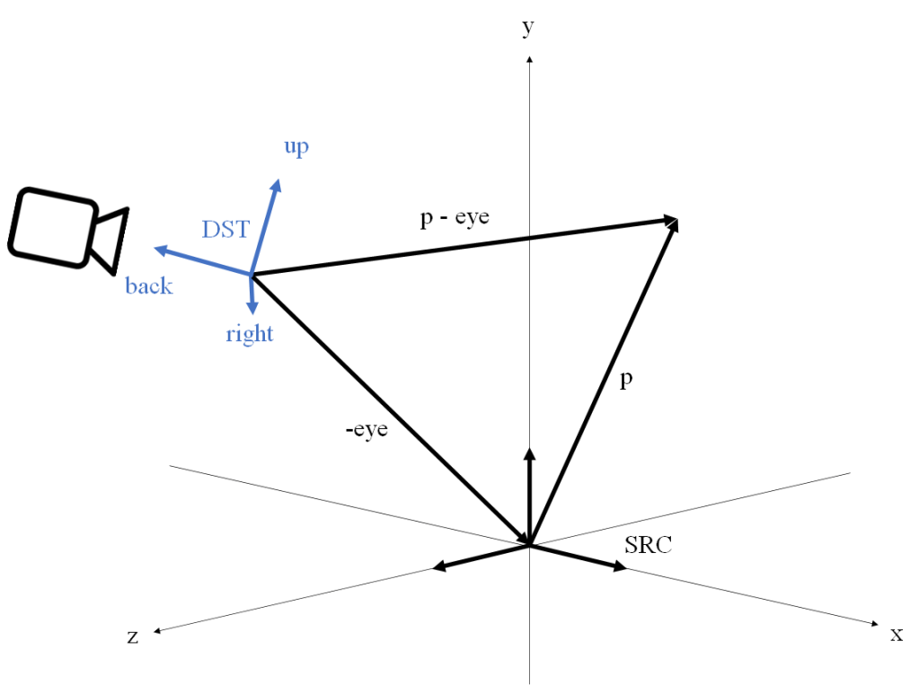
Geometric interpretation of the `lookAt()` matrix

The following figure illustrates the coordinate conversion from the world frame to view frame. Following the previous argument, the geometric interpretation is that we are computing the vector $p - eye$ expressed by its coordinates in the canonical base $SRC$ , and then converting its coordinates to the base $DST$ .

Figure 3. The p – eye vector is computed in SRC and then converted to DST

However, looking at the way the lookAt matrix is built, there’s an alternative geometric interpretation that we could make. Note that if we define the alternative translation matrix

$T' = \begin{pmatrix} 1 & 0 & 0 & -right . eye \\ 0 & 1 & 0 & -up . eye \\ 0 & 0 & 1 & -back . eye \\ 0 & 0 & 0 & 1 \end{pmatrix}$

Then the following matrix multiplication yields the same matrix $M$ defined previously:

$M = T' * R = \begin{pmatrix} right_x & right_y & right_z & -right . eye \\ up_x & up_y & up_z & -up . eye \\ back_x & back_y & back_z & -back . eye \\ 0 & 0 & 0 & 1 \end{pmatrix}$

You can do the multiplication in a sheet of paper to confirm this. Note this is similar to the multiplication from before except that now we apply the linear component first, and translate afterwards using a different translation vector. What does this mean? Remember the geometric meaning of the dot product. When we compute the dot product of a vector $a$ and a unit vector $b$ , this gives us the coordinate of $a$ over $b$ . The translation $T'$ is a translation by the vector $(-right.eye, -up.eye, -back.eye)$ , but this vector is nothing but the coordinates of $-eye$ in the orthonormal base $\{right, up, back\}$ . In other words, the expression $T' * R$ is equivalent to converting the coordinates of the point $p$ from $SRC$ to $DST$ , and then adding $-eye$ expressed in $DST$ . The result is the same displacement vector $p - eye$ that we computed earlier, expressed in $DST$ . The following figure illustrates this. It’s similar to the previous figure, but no we show $-eye$ instead of $eye$ .